


Enameled wire (also known as magnet wire or winding wire), as the core conductor material for electromagnetic components—including transformers, inductors, relays, electromagnets, motors, solenoids, loudspeaker voice coils, switch-mode power supplies (SMPS), induction heating systems, and wireless charging devices—requires precise calculation of the number of turns (Turns) to ensure optimal electromagnetic performance, electrical parameters, thermal characteristics, reliability, and cost-efficiency. Insufficient turns may result in magnetic flux density saturation, excessive temperature rise, inadequate output voltage, low inductance, and excessive ripple; excessive turns may increase copper loss, enlarge physical volume, raise manufacturing cost, elevate leakage inductance, increase distributed capacitance, and degrade frequency response.
Turn calculation for enameled wire is fundamentally an interdisciplinary engineering problem integrating electromagnetism, circuit theory, ferromagnetics, and mechanical winding processes, involving key variables such as the transformer voltage equation, inductor energy equation, magnetic circuit Ohm’s law, Ampère’s circuital law, coil geometric parameters, enamel insulation class, winding window fill factor, and current density (J).
This article systematically elaborates the fundamental principles of enameled wire turn calculation; turns-per-volt (TPV) calculation for transformers; primary and secondary winding turn calculation for transformers; turn calculation for air-core inductor coils (single-layer and multi-layer); turn calculation for magnetic-core coils (ferrite, silicon steel laminations, iron powder cores); turn calculation for relays and electromagnets; stator and rotor turn calculation for motors; turn calculation for loudspeaker voice coils and high-frequency coils; enameled wire diameter selection and current density; coil geometric parameters and window fill ratio; turn accuracy correction factors (skin effect, proximity effect, temperature, saturation); practical calculation examples (50 Hz power-frequency transformer, audio-frequency inductor, SMPS high-frequency inductor, toroidal common-mode inductor); and turn verification and fine-tuning—providing transformer engineers, inductor design engineers, motor engineers, enameled wire application engineers, and electronics engineers with a comprehensive, accurate, and actionable guide to turn calculation and wire selection.
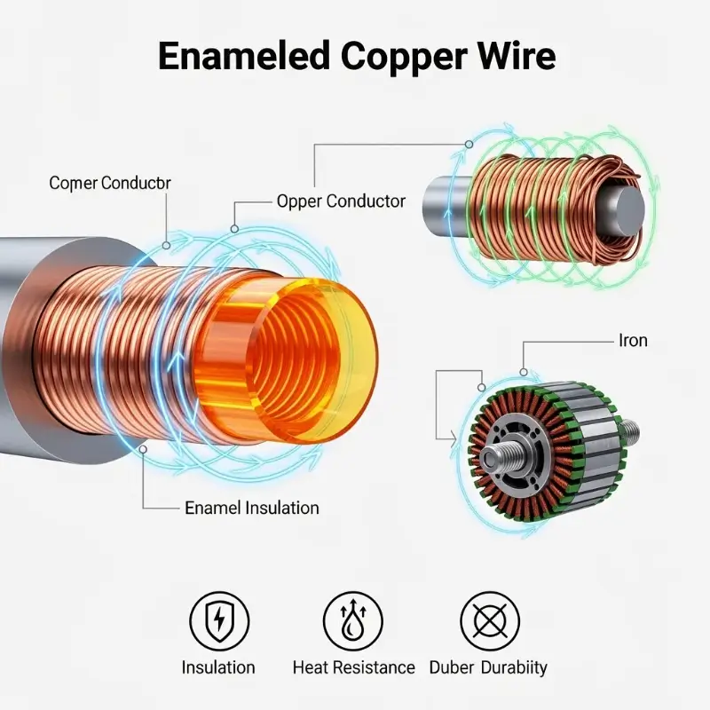
Fundamental Principles of Enameled Wire Turn Calculation
Enameled wire turn calculation is not merely the application of a single formula but rather a multi-variable engineering problem grounded in fundamental electromagnetic laws.
Physical Significance of Turns
The number of turns (N) is the fundamental parameter quantifying electromagnetic coupling strength in a coil:
- Each turn: cuts magnetic flux lines to generate induced electromotive force (EMF)
- Increasing turns: superimposes EMF, increases inductance quadratically (L ∝ N²), and augments magnetomotive force (MMF = N × I)
- Relationship between turns and voltage: Transformer V = 4.44 × f × N × B × A
- Relationship between turns and inductance: L = N² × AL (core inductance factor)
- Relationship between turns and magnetomotive force: F = N × I (ampere-turns)
Fundamental Electromagnetic Laws
Turn calculation relies on the following foundational electromagnetic laws:
Faraday’s Law of Electromagnetic Induction:
- Induced EMF: e = –N × dΦ/dt
- Under sinusoidal steady-state conditions: E = 4.44 × f × N × Bm × A
Lenz’s Law:
- Direction of induced current opposes changes in magnetic flux
- Determines coil dot polarity (terminal A / terminal B)
- Influences transformer phase relationship
Ampère’s Circuital Law:
- For any closed path: ∮H·dl = N × I
- Simplified for uniform magnetic circuits: H × l = N × I
- Magnetomotive force F = N × I
Magnetic Circuit Ohm’s Law:
- Magnetic flux Φ = F / Rm (where Rm is magnetic reluctance)
- Magnetic reluctance Rm = l / (μ × A)
- Relationships: F = H × l = B × l / μ = Φ × Rm
Inductor Energy Storage Equation:
- Stored energy: W = (1/2) × L × I²
- Magnetic energy density: w = B² / (2μ)
- Core-based inductance: L = N² × AL
Core Input Parameters for Turn Calculation
Any turn calculation requires explicit definition of the following inputs:
- Application type (transformer, inductor, motor, relay)
- Operating frequency (f, Hz)
- Operating voltage (V, V) or target inductance (L, H)
- Core material and geometric dimensions (B or AL)
- Operating current (I, A) or power rating (P, W)
- Temperature rise limit (ΔT, K)
- Duty cycle (D, 0–1)
- Enameled wire diameter (d, mm)
- Bobbin dimensions (inner diameter, outer diameter, height)
Turns-Per-Volt (TPV) Calculation for Transformers (Power-Frequency / General Purpose)
Turns-per-volt (TPV) is a core parameter in transformer design, determining the primary-to-secondary turn ratio.
Basic Formula: Turns-Per-Volt (TPV)
Standard Formula:
- TPV = N / V = 1 / (4.44 × f × Bm × A)
- V = 4.44 × f × N × Bm × A
- Rearranged: N = V / (4.44 × f × Bm × A)
Parameter Definitions:
- N: Number of turns
- V: Voltage (V, RMS)
- f: Frequency (Hz)
- Bm: Peak magnetic flux density (T, tesla)
- A: Effective core cross-sectional area (m²)
- 4.44: Sinusoidal waveform coefficient (π/√2 × √2)
TPV Calculation Across Different Frequencies
50 Hz Power-Frequency (China, Europe, India, Australia, etc.):
- TPV = 1 / (4.44 × 50 × B × A) = 1 / (222 × B × A)
- Example: B = 1.2 T, A = 1×10⁻³ m² = 10 cm²
- TPV = 1 / (222 × 1.2 × 0.001) = 3.76 turns/V
60 Hz Power-Frequency (USA, Japan, Canada, Brazil, etc.):
- TPV = 1 / (4.44 × 60 × B × A) = 1 / (266.4 × B × A)
- Example: B = 1.2 T, A = 1×10⁻³ m²
- TPV = 1 / (266.4 × 1.2 × 0.001) = 3.13 turns/V
400 Hz Medium-Frequency (Aviation, military, marine applications):
- TPV = 1 / (4.44 × 400 × B × A) = 1 / (1776 × B × A)
- Example: B = 1.0 T, A = 1×10⁻³ m²
- TPV = 1 / (1776 × 1.0 × 0.001) = 0.563 turns/V
- Advantage: Core and coil size reduced significantly; weight reduction by 5–10×
High-Frequency (kHz-range, SMPS, Inductors):
- Applicable to ferrite cores (B = 0.2–0.4 T)
- Frequency range: 20–500 kHz
- TPV = 1 / (4.44 × f × B × A)
- Example: f = 50 kHz, B = 0.3 T, A = 1 cm² = 1×10⁻⁴ m²
- TPV = 1 / (4.44 × 50000 × 0.3 × 0.0001) = 1.50 turns/V
Selection of Magnetic Flux Density (B)
Selection of B determines core utilization efficiency and saturation margin:
| Application | Frequency | Recommended B (T) | Saturation Margin |
|---|---|---|---|
| 50 Hz silicon steel laminated core | 50 Hz | 1.2–1.5 | 30–40% |
| 50 Hz grain-oriented silicon steel | 50 Hz | 1.5–1.7 | 20–30% |
| 60 Hz silicon steel laminated core | 60 Hz | 1.2–1.5 | 30–40% |
| 400 Hz silicon steel core | 400 Hz | 1.0–1.2 | 20–30% |
| MnZn ferrite | 1–100 kHz | 0.3–0.4 | 30–50% |
| NiZn ferrite | 1–100 MHz | 0.1–0.2 | 30–50% |
| Iron powder core | DC–100 kHz | 0.5–1.0 | 30–40% |
| Permalloy | 1–50 kHz | 0.8–1.2 | 30–50% |
| Amorphous alloy | 50 Hz–10 kHz | 1.0–1.4 | 30–40% |
| Nanocrystalline alloy | 1–100 kHz | 1.0–1.2 | 30–50% |
Calculation of Effective Core Cross-Sectional Area (A)
A denotes the effective magnetic flux cross-sectional area of the core limb or center leg:
E-Core:
- A = (center leg width × stack height) × stacking factor
- Stacking factor K = 0.85–0.95 (laminations: 0.85–0.92; wound silicon steel: 0.95)
- Example: center leg = 20 mm, stack height = 30 mm, K = 0.92
- A = 20 × 30 × 0.92 = 552 mm² = 5.52 cm²
Toroidal Core:
- A = (D_outer – D_inner) × h / 2
- Actual effective area must account for magnetic flux distribution.
- Example: inner diameter 20 mm, outer diameter 40 mm, height 15 mm
- A = (40 – 20) × 15 / 2 = 150 mm² = 1.5 cm²
Pot Core:
- A = π × (D/2)²
- Effective area must also consider the ratio of center leg cross-section to window area.
Transformer Turns Per Volt (TPV) Calculation Examples
Example 1: Small 220 V → 12 V Transformer, 50 Hz
- Core: EI-type, center leg 19 mm, stack height 35 mm, stacking factor K = 0.92
- A = 19 × 35 × 0.92 = 611.8 mm² ≈ 6.12 cm²
- Selected B = 1.2 T
- TPV = 1 / (4.44 × 50 × 1.2 × 6.12×10⁻⁴) = 1 / 0.163 = 6.13 turns/V
Accounting for 5–10% loss margin:
- Actual TPV = 6.13 × 1.05 = 6.44 turns/V
- Primary (220 V): N₁ = 220 × 6.44 = 1417 turns
- Secondary (12 V): N₂ = 12 × 6.44 = 77 turns
Example 2: Small 110 V → 24 V Transformer, 60 Hz
- Core: EI-type, center leg 16 mm, stack height 25 mm, stacking factor K = 0.92
- A = 16 × 25 × 0.92 = 368 mm² = 3.68 cm²
- Selected B = 1.2 T
- TPV = 1 / (4.44 × 60 × 1.2 × 3.68×10⁻⁴) = 1 / 0.118 = 8.51 turns/V
Actual TPV = 8.51 × 1.06:
- Primary (110 V): N₁ = 110 × 9.02 = 992 turns
- Secondary (24 V): N₂ = 24 × 9.02 = 216 turns
Primary and Secondary Turn Calculation for Transformers
The turns ratio (Turns Ratio) of a transformer equals its voltage ratio.
Fundamental Principle
Ideal Transformer Voltage Equation:
- V₁ / V₂ = N₁ / N₂
- V₁ / V₂ = I₂ / I₁ (power conservation)
Practical Considerations:
- Copper loss (IR voltage drop): secondary voltage lower than theoretical value
- Core loss (eddy current and hysteresis losses): increased primary current
- Leakage inductance (leakage flux): coupling coefficient < 1
- Overall efficiency: η = 0.85–0.98
Single-Phase Transformer Design Procedure
Step 1: Determine Rated Parameters
- Power rating P (VA), voltages V₁/V₂, frequency f
- Power factor PF, efficiency η
Step 2: Calculate Rated Currents
- Primary current: I₁ = P / (V₁ × η × PF)
- Secondary current: I₂ = P / (V₂ × η × PF)
Step 3: Select Core
- Core cross-sectional area: A = K × √P (K = 1.0–1.5, empirical coefficient)
- Example: P = 100 VA, A = 1.2 × √100 = 12 cm²
Step 4: Calculate Turns Per Volt (TPV)
- Selected B = 1.2–1.5 T
- TPV = 1 / (4.44 × f × B × A)
Step 5: Calculate Primary Turns
- N₁ = V₁ × TPV
- Round to nearest multiple of 5 or exact integer turn count
Step 6: Calculate Secondary Turns
- N₂ = V₂ × TPV × 1.05 (to compensate for copper-loss voltage drop, 5%)
Step 7: Calculate Wire Diameter
- Primary: d₁ = 1.13 × √(I₁ / J)
- Secondary: d₂ = 1.13 × √(I₂ / J)
- Current density J = 2.5–5 A/mm²
Step 8: Verify Window Fill Factor
- Total copper cross-sectional area / window area ≤ 0.4–0.5
- If exceeded, select larger core
Three-Phase Transformer Turn Calculation
Voltage Relationships:
- Line voltage: V_L = √3 × V_phase (star connection)
- V_L = V_phase (delta connection)
- Turn calculation based on phase voltage; TPV identical to single-phase case
Current Relationships:
- I_L = I_phase (star connection)
- I_L = √3 × I_phase (delta connection)
Magnetic Circuit Calculation:
- Three-phase cores: three-limb, five-limb, or shell-type
- Flux per limb: B identical to single-phase case
Air-Core Inductor Turn Calculation
Air-core inductors have no magnetic core; inductance is determined solely by coil geometry. Turn calculation relies on Wheeler’s formula, modified Wheeler’s formula, or empirical formulas.
Single-Layer Air-Core Inductor (Wheeler’s Formula)
Wheeler’s Formula (Single-Layer Cylindrical Coil):
- L (μH) = (D² × N²) / (1029 × L_coil + 254 × D)
- L (nH) = (D² × N²) / (1029 × L_coil + 254 × D) × 1000
- D: average coil diameter (mm)
- L_coil: coil length (mm)
- N: number of turns
Turn Inversion Formula:
- N = √(L × (1029 × L_coil + 254 × D) / D²)
Accuracy:
- Applicable to: close-wound or spaced single-layer coils
- Accuracy: ±3–5%
- Frequency range: DC–30 MHz
Multi-Layer Air-Core Inductor (Brooks Inductance Formula)
Brooks Formula (Multi-Layer Coil):
- L (μH) = (0.0251 × D × N² × (D/2)) / ((W + 0.46 × D) × ln(8 × D/d) − 2.0 × (W + 0.46 × D) × d/D)
- D: average diameter (mm)
- N: number of turns
- W: coil width (mm)
- d: wire diameter (mm)
Simplified Multi-Layer Formula:
- L (μH) = (R_avg² × N² × 9.87×10⁻³) / (6 × R_avg + 9 × L_coil + 10 × W)
General Multi-Layer Formula:
- L (mH) = (0.08 × D² × N² × 10⁻³) / (3D + 9W + 10H)
- D: coil inner diameter (cm)
- N: number of turns
- W: coil width (cm)
- H: coil height (cm)
Air-Core Coil Turn Calculation Examples
Example 1: Single-Layer RF Choke, 1 μH @ 10 MHz
- Bobbin: diameter 5 mm (D = 5 mm), length 10 mm
- Enameled wire: AWG 30 (d = 0.255 mm)
- L_coil = 10 mm, D = 5 mm
- L(μH) = (D² × N²) / (1029 × L_coil + 254 × D)
- 1 = (5² × N²) / (1029 × 10 + 254 × 5)
- 1 = 25 × N² / (10290 + 1270)
- 1 = 25 × N² / 11560
- N² = 11560 / 25 = 462.4
- N = 21.5 → rounded to 22 turns
Example 2: Multi-Layer Audio Crossover Inductor, 5 mH
- Bobbin: inner diameter 20 mm, length 30 mm, width 25 mm
- D = 20 mm = 2 cm, W = 2.5 cm, H = 3 cm
- Enameled wire: AWG 18 (d = 1.024 mm)
- L(mH) = (0.08 × D² × N² × 10⁻³) / (3D + 9W + 10H)
- 5 = (0.08 × 2² × N² × 10⁻³) / (3×2 + 9×2.5 + 10×3)
- 5 = (0.00032 × N²) / (6 + 22.5 + 30)
- 5 = 0.00032 × N² / 58.5
- N² = 5 × 58.5 / 0.00032 = 914062.5
- N = 956 → rounded to 960 turns
Magnetic-Core Inductor Turn Calculation
Magnetic-core inductors rely on the core’s AL value (inductance factor); turn calculation is straightforward and precise.
AL Value (Inductance Factor)
Definition:
- AL = L / N², units nH/T² or μH/T²
- Inductance produced when one turn is wound on the core
- Determined by core geometry and permeability
Relationship:
- L = N² × AL
- N = √(L / AL)
Typical AL Value Range:
| Core Type | AL Value (nH/T²) |
|---|---|
| T25-X6K Ferrite | 200–500 |
| T50-X6K Ferrite | 800–1500 |
| EE25 Ferrite | 1000–2500 |
| EE40 Ferrite | 3000–6000 |
| ETD29 Ferrite | 2500–4500 |
| ETD49 Ferrite | 5000–9000 |
| PQ20 Ferrite | 1500–3000 |
| PQ40 Ferrite | 5000–10000 |
| Iron Powder Core T80-X2 | 60–100 |
| Silicon Steel EI19 | 1000–2000 |
Core Inductance Turn Calculation Formula
Basic Formula:
- N = √(L / AL)
- N = √(L (μH) / AL (μH/T²))
- N = √(L (nH) / AL (nH/T²))
Example 1: EE25 Ferrite Core, 1 mH Output
- Select EE25-PC40 material, AL = 1800 nH/T²
- N = √(1×10⁶ nH / 1800) = √555.6 = 23.6 → Round up to 24 turns
- Verification: L = 24² × 1800 = 576000 nH = 576 μH (too low; requires more precise AL selection)
- Re-select AL = 1700: N = √(1×10⁶ / 1700) = 24.3 → Round up to 25 turns
- L = 25² × 1700 = 1062500 nH = 1.0625 mH ✓
Example 2: ETD49 Switching Power Supply Filter Inductor, 500 μH @ 100 kHz
- Select ETD49-N87 material, AL = 5500 nH/T² (calculated value)
- N = √(500×10³ / 5500) = √90.9 = 9.5 → Round up to 10 turns
- Verification: L = 10² × 5500 = 550000 nH = 550 μH ✓
AL Value for Gapped Cores
Gapped cores are used to prevent DC saturation and store energy:
AL Calculation for Gapped Cores:
- Total magnetic reluctance: R_m_total = R_m_core + R_m_gap
- AL = 1 / R_m_total
- Gap dominates (small core, large gap)
Equation-Based Method:
- N = √(L × I² × 10⁹ / (B_max² × A) × 8.85×10⁻¹²)
- Simplified: N × I_max = B_max × A × 10⁶ / √(L × 10³)
Power Inductor Example: Energy Storage 100 mJ, Operating Current 10 A
- L = 0.5 × 10⁻² H × (I / I_max)² = ?
- Given: Energy E = (1/2) × L × I² = 100 mJ
- L = 2 × E / I² = 2 × 0.1 / 100 = 2 mH
- Core EE30, core AL = 2200 nH/T², N = √(2000000 / 2200) = 30 turns
Relay and Electromagnet Turn Calculation
Turn calculation for relays, contactors, solenoid valves, and electromagnets is based on ampere-turns (NI) and required magnetomotive force (MMF).
Basic Principle of Attractive Force
Maxwell Suction Formula:
- F = B² × A / (2 × μ₀)
- B: Flux density in air gap (T)
- A: Cross-sectional area of air gap (m²)
- μ₀: Permeability of free space (4π × 10⁻⁷ H/m)
- F: Attractive force (N)
Simplified Form:
- F = (B² × A) / (2 × μ₀)
- F ≈ 400000 × B² × A (SI units, B in T, A in m²)
Ampere-Turn Calculation
Magnetomotive Force Equation:
- N × I = Φ × R_m = H × l / μ_r + H_gap × l_gap × μ₀
- Typically gap-dominated: N × I ≈ H_gap × l_gap = B × l_gap / μ₀
Simplified Calculation:
- N × I = B × l_gap / μ₀ = B × l_gap × 0.8 × 10⁶ (A·T/m)
- Example: l_gap = 0.5 mm, B = 0.3 T
- N × I = 0.3 × 0.5 × 10⁻³ × 0.8 × 10⁶ = 120 A·T
Relay Turn Calculation Example
Example: 12 V DC Relay
- Operating voltage: 12 V DC
- Target coil resistance: R = 200 Ω
- Coil current: I = V / R = 12 / 200 = 0.06 A = 60 mA
- Required attractive force: F = 2 N
- Air gap: l_gap = 0.3 mm
- Pole face area: A = 50 mm² = 5×10⁻⁵ m²
- Target B = 0.2 T
- Required ampere-turns: N × I = 0.2 × 0.3 × 10⁻³ × 0.8 × 10⁶ = 48 A·T
- Turns: N = 48 / 0.06 = 800 turns
Wire diameter selection:
- Current density J = 5 A/mm²
- d = 1.13 × √(I/J) = 1.13 × √(0.06/5) = 1.13 × 0.1095 = 0.124 mm
- Select AWG 36 (0.127 mm) or AWG 37 (0.113 mm)
Resistance verification:
- AWG 36: Resistance 13.8 Ω/m, ~5 m for 800 turns, R = 13.8 × 5 = 69 Ω
- Redesign: R_target = 200 Ω, length L = R × π × r² × 58×10⁶ / ρ
- Select longer or finer enameled wire: AWG 39 (0.09 mm), R = 26.4 Ω/m × 5 m = 132 Ω
- Select AWG 40 (0.08 mm), R = 35 Ω/m × 8 m = 280 Ω (close to 200 Ω)
Solenoid Valve Turn Calculation
DC Solenoid Valve:
- Coil power: P = V² / R
- Target power: P_coil
- Target resistance: R = V² / P_coil
- Turn calculation same as relay
- N = √(R × π × r² × 58×10⁶ × N) … iterative solution required
Example: 24 V Solenoid Valve
- V = 24 V, P = 8 W
- R_target = V² / P = 576 / 8 = 72 Ω
- I = P / V = 8 / 24 = 0.333 A = 333 mA
- Ampere-turns: N × I = 60 A·T (based on air-gap magnetic circuit)
- N = 60 / 0.333 = 180 turns
Wire diameter:
- J = 5 A/mm²
- d = 1.13 × √(0.333/5) = 1.13 × 0.258 = 0.292 mm
- Select AWG 29 (0.286 mm) or AWG 28 (0.320 mm)
Motor Stator and Rotor Turn Calculation
Motors represent the largest application segment for enameled wire; turn calculation involves power, voltage, speed, number of poles, and efficiency.
DC Motor
Back-EMF Equation:
- E = k × Φ × N × ω
- E: Back-EMF (V)
- Φ: Flux per pole (Wb)
- N: Total number of conductors (note: N denotes conductor count in motors, whereas T denotes turns)
- ω: Angular velocity (rad/s)
- k: Constant (depends on winding configuration)
Simplified Form:
- N = E × 60 × a / (k × Φ × p × n)
- p: Number of pole pairs
- n: Speed (rpm)
- a: Number of parallel paths
AC Induction Motor
Turns per Phase:
- N_ph = k_E × V_ph × 10⁸ / (4.44 × f × Φ × K_w)
- k_E: EMF constant (0.85–0.95)
- V_ph: Phase voltage (V)
- K_w: Winding factor (0.85–0.96)
- Φ: Flux per pole (Mx, 1 Mx = 10⁻⁸ Wb)
- f: Supply frequency (Hz)
Example: 1.5 kW Three-Phase Induction Motor, 380 V, 50 Hz
- V_ph = 380 / √3 = 220 V
- Φ = 4.5×10⁻³ Wb
- K_w = 0.92
- k_E = 0.92
- N_ph = 0.92 × 220 × 10⁸ / (4.44 × 50 × 4.5×10⁻³ × 0.92) = 0.92 × 2.2×10¹⁰ / 184 = 1.1×10⁸ ≈ 110 turns/phase
AC Synchronous Motor
Turns per phase (similar to induction motor):
- N_ph = V_ph / (4.44 × f × Φ × K_w)
- Short-pitch factor K_p and distribution factor K_d are incorporated into K_w
Brushless DC Motor (BLDC)
Turns per phase:
- N_ph = (E / K_E) × 60 / (n × p)
- E: back EMF (V)
- K_E: back EMF constant (V/krpm)
- n: rated speed (rpm)
- p: number of pole pairs
Voice Coil and High-Frequency Coil Turn Calculations
Voice coils and high-frequency (HF) coils represent high-end applications of magnet wire, where turn count is closely tied to geometric parameters.
Voice Coil Turn Calculation
Basic voice coil parameters:
- Voice coil diameter: d_vc (mm)
- Voice coil length: l_vc (mm)
- Wire diameter: d_w (mm)
- Voice coil turns: N_vc
Relationship between turns and voice coil length:
- l_vc = N_vc × d_w × (1 + enamel thickness ratio)
- Total wire diameter d_total includes insulation layer
- Example: d_w = 0.15 mm (bare copper), d_total = 0.17 mm
- l_vc = 10 mm → N_vc = 10 / 0.17 = 58 turns
Voice coil impedance calculation:
- R = ρ × l_wire / A_wire
- l_wire = π × (D_vc + d_w) × N_vc
- A_wire = π × d_w² / 4
- Example: D_vc = 25 mm, d_w = 0.15 mm, N_vc = 58 turns
- l_wire = π × 25.15 × 58 = 4578 mm = 4.578 m
- R = 0.01724 × 4.578 / (π × 0.15² / 4) = 0.0789 / 0.01767 = 4.47 Ω (theoretical value for copper)
Actual voice coil impedance:
- Typically standardized at 4 Ω, 8 Ω, 16 Ω, or 32 Ω
- Impedance matched to amplifier output
- DC resistance equals 80–90% of nominal impedance
High-Frequency Coil (HF Coil)
Single-layer RF coil:
- L (μH) = (D × N²) / (1029 × L_coil + 254 × D)
- D (mm), L_coil (mm), L (μH)
- N = √(L × (1029 × L_coil + 254 × D) / D²)
Example: 10 μH air-core RF coil at 100 MHz:
- Former diameter D = 10 mm, coil length L_coil = 15 mm
- N = √(10 × (1029 × 15 + 254 × 10) / 100)
- N = √(10 × (15435 + 2540) / 100)
- N = √(10 × 179.75)
- N = √1797.5 = 42.4 → select 42 turns
Skin Depth and Wire Diameter Limitation
Skin depth δ:
- δ = √(ρ / (π × f × μ))
- ρ: resistivity (Ω·m)
- f: frequency (Hz)
- μ: permeability (H/m)
Copper skin depth at 20°C:
| Frequency | Skin depth δ (mm) |
|---|---|
| 50 Hz | 9.36 |
| 1 kHz | 2.10 |
| 10 kHz | 0.66 |
| 100 kHz | 0.21 |
| 1 MHz | 0.066 |
| 10 MHz | 0.021 |
| 100 MHz | 0.0066 |
Practical recommendations:
- Conductor radius should be < 2 × δ at operating frequency
- Otherwise, use Litz wire
- Multiple fine strands reduce AC losses
Magnet Wire Gauge Selection and Current Density
Turn count calculation addresses magnetic field requirements only; actual winding necessitates appropriate magnet wire gauge selection.
Current Density (J) Selection
Current density J = I / A_cross:
- A_cross: cross-sectional area of magnet wire (mm²)
- J: current density (A/mm²)
Typical current density ranges:
| Application | J (A/mm²) | Remarks |
|---|---|---|
| Small transformers | 4–6 | Commercial transformers |
| Large transformers | 2–3.5 | Industrial transformers |
| Power transformers | 3–5 | General-purpose power supplies |
| High-frequency transformers | 2–4 | SMPS, induction heating |
| Relay coils | 5–8 | High power density |
| Solenoid valves | 5–10 | Intermittent duty |
| Motor stators | 4–8 | Medium- and small-size motors |
| Voice coils | 10–30 | Intermittent duty |
Magnet Wire Gauge Calculation
Relationship between wire diameter d and cross-sectional area A:
- A = π × d² / 4
- d = √(4 × A / π) = 1.128 × √A
- Practical approximation: d = 1.13 × √(I / J)
Example: 3 A magnet wire, J = 5 A/mm²:
- A = 3 / 5 = 0.6 mm²
- d = 1.13 × √0.6 = 1.13 × 0.775 = 0.875 mm
- Select AWG 19 (0.912 mm) or AWG 20 (0.813 mm)
Standard Magnet Wire Gauge Reference (including enamel coating)
Metric-to-AWG conversion table:
| Bare copper diameter (mm) | AWG equivalent | Cross-sectional area (mm²) | Resistance (Ω/m at 20°C) | Current rating @ 2.5 A/mm² | Current rating @ 4 A/mm² |
|---|---|---|---|---|---|
| 0.10 | 38 | 0.00785 | 2.196 | 0.020 A | 0.031 A |
| 0.20 | 32 | 0.0314 | 0.549 | 0.079 A | 0.126 A |
| 0.30 | 29 | 0.0707 | 0.244 | 0.177 A | 0.283 A |
| 0.50 | 24 | 0.196 | 0.0876 | 0.491 A | 0.785 A |
| 0.80 | 20 | 0.503 | 0.0342 | 1.257 A | 2.011 A |
| 1.00 | 18 | 0.785 | 0.0219 | 1.963 A | 3.142 A |
| 1.50 | 15 | 1.767 | 0.00975 | 4.418 A | 7.069 A |
| 2.00 | 12 | 3.142 | 0.00549 | 7.854 A | 12.566 A |
Litz Wire (Multi-strand Magnet Wire)
Construction: multiple individually insulated fine wires twisted together
Designation format:
- N × d × S: number of strands × bare copper diameter per strand × lay length
- Example: 100 × 0.10 × 25: 100 strands of 0.10 mm diameter wire, lay length 25 mm
Applications:
- High-frequency transformers (>50 kHz)
- Induction heating (>10 kHz)
- Wireless charging (100 kHz–1 MHz)
- Communication power supplies
Reduces skin effect and proximity effect losses
Coil Geometric Parameters and Window Fill Factor
The winding window must accommodate all turns; the window fill factor determines design feasibility.
Window Fill Factor
Definition:
- K_fill = A_Cu_total / A_window
- K_fill: window fill factor (0–1)
- A_Cu_total: total cross-sectional area of all magnet wires
- A_window: window area of coil bobbin
Typical range:
| Winding Method | K_fill | Application Scenario |
|---|---|---|
| Random winding | 0.40–0.50 | General-purpose |
| Aligned winding | 0.50–0.65 | High-frequency, low-loss applications |
| Litz wire winding | 0.30–0.40 | High-frequency applications |
| Square wire | 0.65–0.75 | High-power-density applications |
| Rectangular wire | 0.70–0.85 | High-frequency transformers, planar transformers |
Window Fill Factor Calculation
Single-layer winding:
- Space occupied per turn: d_total (overall diameter of enameled wire)
- Total number of turns: N
- Coil length: L_coil = N × d_total
- Required window height: H_window ≥ N × d_total
- Verification: H_window × W_window × (1 / d_total) ≥ N
Multi-layer winding:
- Turns per layer: N_layer = W_window / d_total
- Number of layers: n_layers = N / N_layer
- Required height: H_required = n_layers × d_total
- Verification: H_window ≥ H_required
Example: 220 V → 12 V transformer, primary winding with 1,417 turns
- Enameled wire AWG 30: d = 0.255 mm, d_total = 0.290 mm (including insulation film)
- Bobbin window: width = 20 mm, height = 30 mm
- Turns per layer: N_layer = 20 / 0.290 = 69 turns/layer
- Number of layers: n = 1,417 / 69 = 20.5 → 21 layers
- Required height: H = 21 × 0.290 = 6.1 mm
- Actual window utilization: 6.1 / 30 = 20% (excellent design)
End-winding Height and Winding Margin
End-winding space:
- Additional space required at start and end of winding
- Typically 20–30% extra margin
- Total required window height: H_required × 1.25
Turn Count Accuracy Correction and Edge Effects
Theoretical calculations must account for practical deviations to ensure adequate design margin.
Skin Effect Correction
Skin effect-induced AC resistance increase:
- R_AC > R_DC
- R_AC / R_DC = 1 + (1/48) × (r/δ)⁴ (for small r/δ)
- Example: 100 kHz, copper wire diameter = 0.5 mm
- δ = 0.21 mm, r/δ = 0.25 / 0.21 = 1.19
- R_AC / R_DC ≈ 1 + (1/48) × 1.19⁴ = 1.42
- Practical solution: use enameled wire < 0.2 mm diameter or Litz wire
Proximity Effect Correction
Proximity effect:
- Adjacent conductor currents induce additional eddy currents
- Significant impact in multi-layer windings
- Mitigation: reduce turns per layer, increase inter-turn spacing, or employ Litz wire
Temperature Correction
Resistance temperature coefficient:
- α_Cu = 0.00393 /°C (20–100°C)
- R(T) = R(20°C) × [1 + 0.00393 × (T − 20)]
Inductance temperature stability:
- Ferrite cores: temperature coefficient = 1,000–3,000 ppm/°C
- Silicon steel laminations: temperature coefficient = 500–1,000 ppm/°C
- Iron powder cores: temperature coefficient = 100–500 ppm/°C
Saturation Margin
Flux density saturation margin:
- B_op = B_sat / (1 + saturation margin)
- 50 Hz silicon steel: B_sat = 1.8–2.0 T, B_op = 1.2–1.5 T (margin = 30–40%)
- Ferrite PC40: B_sat = 0.5 T @ 25°C, B_op = 0.2–0.3 T (margin = 50–60%)
Leakage Inductance Correction
Leakage inductance (L_Lk):
- Primarily caused by incomplete magnetic coupling between windings
- L_Lk / L ≈ 1–10% (for tightly coupled windings)
- Impact: switching spikes, EMI generation
- Reduction methods: interleaved (sandwich) winding, sectional winding
Distributed Capacitance Correction
Distributed capacitance (C_d):
- Inter-turn and inter-layer capacitance
- C_d ≈ 5–50 pF (typical)
- Forms resonant circuits at high frequencies
- Mitigation: sectional winding, reduced turns per layer
Final Turn Count After Corrections
Final turn count:
- N_actual = N_theoretical × (1 + ε_total)
- ε_total: total correction factor (5–10%)
- Example: N_th = 100 turns, ε = 8%
- N_actual = 100 × 1.08 = 108 turns
Turn Count Calculation Examples Summary
Example 1: 50 Hz EI Power Transformer
Requirements:
- Input: 220 V, 50 Hz
- Output: 12 V / 5 A
- Efficiency: 85%
- Temperature rise: 60 K
- Duty cycle: continuous
Step 1: Power rating:
- P_out = 60 W
- P_in = 60 / 0.85 = 70.6 W
Step 2: Current calculation:
- I_2 = 5 A
- I_1 = 70.6 / 220 = 0.32 A
Step 3: Core selection:
- A = 1.2 × √P = 1.2 × √70.6 = 10.07 cm²
- Selected core: EI 96, center leg = 24 mm, stack height = 45 mm
- A_actual = 24 × 45 = 1,080 mm² = 10.8 cm²
- K_fill_core = 0.92
- A_eff = 1,080 × 0.92 = 994 mm² = 9.94 cm²
Step 4: Turns per volt (TPV):
- B = 1.2 T
- TPV = 1 / (4.44 × 50 × 1.2 × 9.94×10⁻⁴)
- TPV = 1 / (4.44 × 50 × 1.1928×10⁻³)
- TPV = 1 / 0.2648
- TPV = 3.78 turns/V
Step 5: Primary turns:
- V_1 = 220 V
- N_1 = 220 × 3.78 × 1.08 (8% loss compensation) = 898 turns
- Rounded N_1 = 900 turns
Step 6: Secondary turns:
- V_2 = 12 V × 1.08 = 12.96 V (voltage drop compensation)
- N_2 = 12.96 × 3.78 = 49 turns
- Rounded N_2 = 50 turns
Step 7: Wire gauge selection:
- Primary current density J = 4 A/mm²: d_1 = 1.13 × √(0.32/4) = 0.32 mm
- Selected: AWG 28 (0.32 mm)
- Secondary current density J = 4 A/mm²: d_2 = 1.13 × √(5/4) = 1.27 mm
- Selected: AWG 16 (1.291 mm)
Step 8: Window fill verification:
- Bobbin window: width = 28 mm, height = 50 mm
- A_total = N_1 × π × d_1² / 4 + N_2 × π × d_2² / 4
- A_Cu = 900 × 0.0804 + 50 × 1.3096 = 72.4 + 65.5 = 137.9 mm²
- A_window = 28 × 50 = 1,400 mm²
- K_fill = 137.9 / 1,400 = 9.85%
- Excellent window utilization
Example 2: SMPS 50 kHz High-Frequency Transformer
Requirements:
- Input: 310 V DC (rectified 220 V AC)
- Output: 24 V / 5 A
- Efficiency: 92%
- Operating frequency: 50 kHz
- Core: EE30-PC40
Step 1: Core parameters:
- EE30: A_e = 109 mm² = 1.09×10⁻⁴ m²
- A_L = 2,300 nH/T² = 2.3 μH/T²
Step 2: Flux density selection:
- f = 50 kHz, suitable for PC40
- B_max = 0.25 T @ 100°C
Step 3: Turns per volt (TPV):
- TPV = 1 / (4.44 × 50,000 × 0.25 × 1.09×10⁻⁴)
- TPV = 1 / (4.44 × 50,000 × 2.725×10⁻⁵)
- TPV = 1 / 6.05
- TPV = 0.165 turns/V
Step 4: Primary turns:
- V₁ = 310 V (including ripple)
- N₁ = 310 × 0.165 × 1.08 = 55.2
- Select N₁ = 55 turns
Step 5: Secondary Turns:
- V₂ = 24 / 0.92 = 26.1 V
- N₂ = 26.1 × 0.165 = 4.3 → select 5 turns
- N₂/N₁ = 5/55 = 1/11
- V₂_actual = 310 / 11 = 28.2 V (higher than target; duty cycle adjustment required)
Step 6: Wire Gauge:
- I₁ = 60 × 0.92 / 0.85 / 310 ≈ 0.21 A (actual primary RMS current)
- I₂ = 5 A
- J = 4 A/mm²
- d₁ = 1.13 × √(0.21/4) = 0.26 mm (AWG 30 Litz wire)
- d₂ = 1.13 × √(5/4) = 1.27 mm (AWG 16)
Step 7: Litz Wire:
- f = 50 kHz, skin depth δ = 0.296 mm
- Strand diameter ≤ 2δ = 0.592 mm
- Select 0.10 mm strand Litz wire, 50 strands (total equivalent diameter 1.0 mm)
Example 3: Toroidal Common-Mode Choke
Requirements:
- Inductance: 5 mH
- Frequency range: 10 kHz–30 MHz
- Impedance: ≥500 Ω @ 30 MHz
- Core: MnZn ferrite toroid
Step 1: Core Selection:
- T25 × 12.5 × 12.5 (OD 25 mm, ID 12.5 mm, height 12.5 mm)
- Aₗ = 2000 nH/T²
Step 2: Turns Calculation:
- N = √(5×10⁶ / 2000) = √2500 = 50 turns
Step 3: Impedance Verification:
- At 30 MHz: Xₗ = 2π × 30×10⁶ × 5×10⁻³ = 942 kΩ
- However, due to ferrite core losses and distributed capacitance, impedance peak occurs at ~1–10 kHz
- At 10 kHz: Xₗ = 314 Ω
- At 100 kHz: Xₗ = 3142 Ω
- At 1 MHz: Xₗ = 31416 Ω (practically 1000–5000 Ω)
Step 4: Wire Gauge:
- Rated current I = 1 A
- J = 5 A/mm²
- d = 1.13 × √(1/5) = 0.51 mm
- Select AWG 24 (0.511 mm)
Example 4: DC Relay
Requirements:
- Voltage: 12 V DC
- Pull force: 1.5 N
- Air gap: 0.4 mm
- Pole face area: 40 mm²
- Operating current: <100 mA
Step 1: Magnetomotive Force (MMF):
- B_target = 0.15 T
- H_gap = B / μ₀ = 0.15 / (4π×10⁻⁷) = 119,366 A/m
- l_gap = 0.4 mm = 4×10⁻⁴ m
- NI = H × l_gap = 119,366 × 4×10⁻⁴ = 47.7 A·T
Step 2: Turns Calculation:
- Coil current I = 0.08 A (<100 mA)
- N = 47.7 / 0.08 = 596 → select 600 turns
Step 3: Wire Gauge:
- J = 5 A/mm²
- d = 1.13 × √(0.08/5) = 0.143 mm
- Select AWG 35 (0.142 mm)
Step 4: Coil Resistance:
- AWG 35: R = 9.06 Ω/m; 600 turns ≈ 3 m
- R_coil = 9.06 × 3 = 27.2 Ω
- I_actual = 12 / 27.2 = 0.44 A (excessive)
- Redesign: reduce wire gauge
Step 5: Iterative Design:
- Target R = 12 / 0.08 = 150 Ω
- Length = 3 m
- Unit resistance R_u = 150 / 3 = 50 Ω/m
- Select AWG 42 (0.0635 mm), R_u = 53.4 Ω/m
- d = 0.0635 mm, J = 0.08 / (π × 0.0635² / 4) = 25.3 A/mm² (excessive)
- Select AWG 38 (0.10 mm), R_u = 22 Ω/m, length = 150/22 = 6.8 m
- d = 0.10 mm, J = 0.08 / 0.00785 = 10.2 A/mm² (still high)
- Select AWG 39 (0.09 mm), J = 12.6 A/mm² (high but acceptable for short-term operation)
- Select AWG 40 (0.08 mm), J = 15.9 A/mm² (high, short-term)
Accepted Solution:
- AWG 40, 1000 turns
- Length ≈ 8 m
- R_coil ≈ 8 × 35 = 280 Ω
- I_actual = 12 / 280 = 43 mA
- NI_actual = 1000 × 0.043 = 43 A·T (below target 47.7)
- Adjustment: increase turns to 1200, length 9.6 m, R = 336 Ω, I = 36 mA, NI = 43 A·T
- Or reduce target: F_target = 1.2 N, NI = 38 A·T, 1100 turns reasonable
Example 5: Voice Coil Winding
Requirements:
- Voice coil diameter: 25 mm
- Voice coil height: 10 mm
- Impedance: 4 Ω
- Conductor: copper round enameled wire
Step 1: Wire Selection:
- Enameled wire diameter d = 0.15 mm (copper), total diameter d_total = 0.17 mm
Step 2: Turns Calculation:
- Turns per layer: N_layer = 10 / 0.17 = 58 turns
- Single-layer winding
- N = 58 turns
Step 3: Wire Length:
- l = π × (D_vc + d) × N = π × (25 + 0.15) × 58 = 4578 mm = 4.578 m
Step 4: Resistance Calculation:
- A = π × 0.15² / 4 = 0.01767 mm²
- R = 0.01724 × 4.578 / 0.01767 = 4.47 Ω (DC resistance)
- AC resistance (accounting for skin effect and voice coil alternating magnetic field): ~5.5–6 Ω (impedance increase ~30%)
- Actual impedance: ~4 Ω (including DC bias adjustment and temperature effects)
Step 5: Power Handling:
- P_max = I² × R = 30² × 4 = 3600 W (peak)
- Continuous rated power P_rated = 10–50 W
Turns Verification and Fine-Tuning
After theoretical calculation, verification via measurement and necessary fine-tuning is mandatory.
DC Resistance Test
Test Method:
- Multimeter ohmmeter function
- Four-wire (Kelvin) method (for precision)
- Temperature correction: R(T) = R(20°C) × [1 + α × (T − 20)]
Acceptance Criteria:
- Measured value vs calculated value: ±5%
- Excessive deviation indicates incorrect turns count, wrong wire gauge, or wiring error
Inductance Test
Test Method:
- LCR meter (at 10 kHz, 1 kHz, 100 kHz)
- Q-meter
- Impedance analyzer
Acceptance Criteria:
- Measured inductance vs target inductance: ±5–10%
- Q factor: ≥30 for high-frequency applications; ≥5 for low-frequency applications
Turns Ratio Test
Test Method:
- Apply known voltage to primary winding
- Measure secondary voltage
- Calculate: N₁/N₂ = V₁/V₂
Acceptance Criteria:
- Deviation: ±1%
Temperature Rise Test
Test Method:
- Full-load operation for 4–8 hours
- Measure temperature after thermal stabilization
- Temperature rise ΔT = T_hot − T_ambient
Acceptance Criteria:
- ΔT < design limit (typically 60–90 K)
Turns Fine-Tuning
Fine-Tuning Methods:
- Above target: reduce turns (remove 1 turn, measure inductance)
- Below target: increase turns (add 1 turn, measure inductance)
- Typical fine-tuning increment: 1–5 turns
Software-Assisted Tools:
- FEMM (2D magnetic field simulation)
- Maxwell 3D
- JMAG
Summary
Turn count calculation for magnet wire is a core issue in electromagnetic engineering. This document’s 12 chapters cover: turns-per-volt calculation for transformers; primary and secondary winding turn calculations for transformers; air-core inductor coil turn calculations (single-layer and multi-layer); magnetic-core coil turn calculations (ferrite, silicon steel laminations); relay and electromagnet turn calculations; motor stator turn calculations; loudspeaker voice coil turn calculations; wire gauge selection and current density; coil geometric parameters and window fill factor; turn count accuracy corrections (skin effect, proximity effect, temperature, saturation, leakage inductance, distributed capacitance); five complete calculation examples (50 Hz power-frequency transformer, SMPS high-frequency transformer, toroidal common-mode inductor, DC relay, voice coil); and turn count verification and fine-tuning.
Key formulae summary:
- Transformer turns per volt: TPV = 1 / (4.44·f·B·A)
- Inductor turns: N = √(L / AL) (magnetic core); N = √(L·(1029·L_coil+254·D)/D²) (Wheeler single-layer)
- Magnetomotive force: N·I = H·l_gap
- Wire diameter: d = 1.13·√(I / J)
Design workflow: Define input parameters (V, f, L, B, AL, I) → calculate theoretical turns → select wire gauge → verify window fill factor → apply corrections (skin effect, proximity effect, temperature, saturation) → incorporate engineering margin → perform empirical validation → finalize fine-tuning. With growing demand—driven by emerging applications such as wireless charging, new-energy vehicles, photovoltaic inverters, energy storage systems, and AI server power supplies—for high-frequency, high-efficiency, and high-power-density transformers, the precision requirements for turn count calculation continue to rise, necessitating an integrated engineering closed loop combining simulation software, empirical validation, and process optimization.